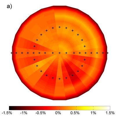
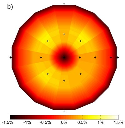
Fig 1: Temperature distribution at the surface of the heating plate (a) and the cooling plate (b) at
, aspect ratio of 2.75 and
. The plots show the relative deviation
and
as a percentage of the total temperature drop between the plates. The crosses indicate the position of the internal temperature sensors. The radial temperature distribution at each segment is a projection of the measured distribution along the horizontal line, whereas the angular distributed temperature sensors are used as basic values.
The free-hanging cooling plate consists of 16 segments with water circulation inside as well. The segments are mounted on a solid steel construction and are separately levelled perpendicular to the vector of gravity. The entire construction with a weight of about 6 tons is mounted on a crane and can be lifted up and down. A small gap between the plate and the sidewall, required to freely move the plate, is hermetically sealed with strips of foam during the experiments. In the present experiments, the temperature of the cooling plate was set between
= 28.8 and 12.4°C with the same accuracy as indicated for the heating plate. The plate distance has been varied from H = 6.30 m to 0.79 m covering aspect ratios between = 1.13 and 9.00. The sidewall of the Rayleigh-Bénard cell is shielded by an active compensation heating system to prevent heat exchange with the surroundings. Electrical heating elements are arranged between an inner and an outer isolation of 16 and 12 cm thickness, respectively. The temperature of these elements is controlled to be equal to the temperature at the inner surface of the wall. The heat loss was checked by setting the temperature of both plates to 30.0°C, the fluid temperature that was maintained in the well-mixed bulk region during our experiments. In the case of a perfectly adiabatic side wall, the fluid temperature has to be exactly the same. The measured values were 29.9°C, a deviation that indicates a very small heat loss not exceeding 0.5% of the convective heat flux in the experiments. For more detailed information see du Puits et al (2007a).
Measurement technique
Local temperature measurements have been carried out inside and outside the boundary layers. Here, boundary layers are referred to as those regions where the temperature increases or decreases from the plate temperature to the temperature of the well-mixed core. It should be noted as well that the typical thickness of this region is of the order of 1 cm in the 6.3 m-high Rayleigh-Bénard cell, at the maximum possible Rayleigh number
with (
denoting the thermal expansion coefficient, the gravitational acceleration and the temperature difference between the hot bottom and the cool top plate, respectively). Therefore, very small, glass encapsulated, microthermistors (temperature-dependent resistors) of size 125 μm were used to probe the temperature field. All measurements were carried out along the central axis of the cylindrical Rayleigh-Bénard cell and cover distances between
. (corresponding to the radius of the microthermistor) and
. The thermistors are connected to the tips of two 0.3 mm supports by 18 μm wires (see figure 2). Due to the strong temperature gradients close to the wall and unlike in the authors' experiments in the past, care was taken to align these connecting wires exactly parallel to the plates and along the iso-surfaces of constant mean temperature in the flow. This prevents measurement errors of the order of a few degrees Kelvin, and the accuracy particularly very close to the plate surfaces could be improved by a factor of about 20 compared to those measurements in the past. Another source of measurement uncertainty is the spatial averaging of the sensor in the high-temperature gradient flow field close to the wall. This issue may distort (linearize) the natural shape of the temperature field inside the boundary layer. In the work reported here, the maximum gradients have been measured at They amount to the mean temperature gradients:
right at the surface of the heating and the cooling plates (see du Puits et al, 2007b). Considering the sensor as a sphere with a diameter of 125 μm the temperature drop across the sensor amounts to
and , respectively, or, expressed in units of the total temperature drop across the boundary layer, to
.
It should be noted here that these values are the absolute maxima at this particular parameter set, while the temperature drop was significantly smaller during the other measurements.
Fig. 2: Set-up of the temperature and the heat flux measurement at the heating plate. The temperature sensor can be moved up and down. The heat flux sensor is mounted using a thermally conducting glue. The upper right picture shows a strongly enlarged photograph of the microthermistor and its attachment at the support.
Before starting the measurements, the sensors were calibrated in a calibration chamber. A resistance temperature detector (RTD) of PT 100 type certified by the Deutsche Kalibrierdienst was used as the reference. The measurement uncertainty of this sensor is specified with 0.02 K in the range between 0 and 100°C. The temperature of the microthermistor in the flow field was determined by measuring its resistance and recomputing the temperature according to the calibration curve. A special bridge with an internal amplifier provided a very low measurement current of
sufficiently small to keep the self-heating of the sensor as low as 10 mK. The bridge was connected to a PC-based multi-channel data acquisition system with a resolution of 10⁻⁴ K and a sampling rate of 200 s⁻¹ (du Puits et al, 2007b).
Available Data
Data available consist of mean and rms temperature profiles on the centreline of the cylinder across the boundary layers at both the cold and heated plates.
Sample plots of selected quantities are available.
| | | |
| 1.13 | 5.20 x 10¹⁰ | G=1.13_Ra=5.20e10 | G=1.13_Ra=5.20e10 |
| 1.25 | 5.18 x 10¹⁰ | G=1.25_Ra=5.18e10 | G=1.25_Ra=5.18e10 |
| 1.50 | 5.25 x 10¹⁰ | G=1.50_Ra=5.25e10 | G=1.50_Ra=5.25e10 |
| 1.75 | 5.26 x 10¹⁰ | G=1.75_Ra=5.26e10 | G=1.75_Ra=5.26e10 |
| 2.00 | 5.26 x 10¹⁰ | G=2.00_Ra=5.26e10 | G=2.00_Ra=5.26e10 |
| 2.25 | 5.20 x 10¹⁰ | G=2.25_Ra=5.20e10 | G=2.25_Ra=5.20e10 |
| 2.50 | 5.19 x 10¹⁰ | G=2.50_Ra=5.19e10 | G=2.50_Ra=5.19e10 |
| 2.75 | 5.20 x 10¹⁰ | G=2.75_Ra=5.20e10 | G=2.75_Ra=5.20e10 |
| 2.75 | 4.00 x 10⁹ | G=2.75_Ra=4.00e09 | G=2.75_Ra=4.00e09 |
| 3.00 | 3.90 x 10⁹ | G=3.00_Ra=3.90e09 | G=3.00_Ra=3.90e09 |
| 4.00 | 3.95 x 10⁹ | G=4.00_Ra=3.95e09 | G=4.00_Ra=3.95e09 |
| 5.00 | 3.85 x 10⁹ | G=5.00_Ra=3.85e09 | G=5.00_Ra=3.85e09 |
| 6.00 | 3.86 x 10⁹ | G=6.00_Ra=3.86e09 | G=6.00_Ra=3.86e09 |
| 7.01 | 3.79 x 10⁹ | G=7.01_Ra=3.79e09 | G=7.01_Ra=3.79e09 |
| 9.00 | 1.31 x 10⁹ | G=9.00_Ra=1.31e09 | G=9.00_Ra=1.31e09 |
Discussion of Results
A selection of the normalized mean temperature profiles at aspect ratios between
are plotted in figure 3. All profiles obtained at one plate turn out to be similar, with the deviation not exceeding 10%. Small deviations visible in the lin-lin representation in the insets might be associated with non-Boussinesq effects due to the change in the temperature drop, which amounts to
in the experiment at
in the
experiment.
While the variation of the fluid properties can be neglected for the minimum temperature difference, it is worth noting that, for example, the heat conductivity λ varies by about 15% across the cell for the highest one. This variation causes the temperature gradients at the surface of the heating and the cooling plates to differ by 15% as well.

")
")
 temperature fluctuations at the heating (a)")
 temperature fluctuations at the cooling (b) plates")